Summary
In the simple version of supply chain management (SCM) the goal for demand forecasting in the tactical decision tier is prediction accuracy. In the wiser version, the purpose is expanded to include an understanding of your demand (demand profiling), bound the level of accuracy possible by using demand history and using this information to support demand and inventory analysis by putting in place programs to enable the firm to adapt to changing conditions. Getting to wiser forecasting requires the use of machine learning (ML) and automated intelligence (AI) combined with deep statistical knowledge imbedded in software with expert system (ES) methods and the use of advanced optimization. This is part of Arkieva’s Swifcast. Besides dramatically improving forecast accuracy by evaluating alternative forecasting methods (ARIMA, Holt-Winters, etc.) and levels of aggregation (product, product and location, product family, etc.), it provides the critical insight – the best you can do with the data that you have. It can also point the way to additional data needed to improve the forecast, how to assess risk, and how best to monitor and track execution (decision tier relevant time response). One of the critical functions in Swifcast is demand profiling.
Most experienced planners can identify the core patterns found in figures 1 to 5 (seasonal, stationary, stationary with correlation with prior demand, jump step, and intermittent). However, the planner might need some help from a seasoned applied statistician. Given the number of time series and the time to do a manual review, manual classification is not feasible. With Swifcast, machine learning and the company do the heavy lifting to classify each time series. This represents a substantial improvement over the historic method using the coefficient of variation which was originally used in chemistry and misused in the supply chain. This blog provides a quick overview of Swifcast and a deeper look at demand profiling. Future blogs will dive into specific aspects in more depth.
Introduction
In the simple version of supply chain management (SCM) the goal for demand forecasting in the Kempf-Sullivan decision tiers 2 or 3 is prediction accuracy based on the smallest “measure of error”. Error is defined as the difference between the predicted value and the observed or historical value per time period and aggregated across time. All aggregation methods involve eliminating the direction of error (using squaring or absolute deviation), some type of averaging, and sometimes the concept of fit and predict.
In the wiser version, the purpose is expanded to include an understanding of your demand (demand profiling), bound the level of accuracy possible using demand history by evaluating the level of forecasting (product, product and location, product family, etc.) and various forecasting methods (exponential smoothing, moving average, robust seasonal, Holt-Winters, ARIMA, Croston, bootstrapping, etc.), and classifying your historic demand to support demand and inventory analysis and put in place programs to enable the firm to adapt to changing conditions. In other words, keeping chaos at bay. Arkieva provides this “wiser” forecasting in Swifcast available on the web. Arkieva uses a synergy of machine learning, automated intelligence, and advanced optimization for statistics to provide this critical function. This work follows the path established in the symposiums on the interface of computer science and statistics.
This blog provides an overview of demand profiling that is a critical component of advanced demand management. To accomplish this requires intermixing methods from Artificial Intelligence (AI) and advanced statistics.
Origins of Demand Profiling in Inventory Management
Historically best in class inventory management classifies demand based on variability into groups, three common ones are:
- Regular demand – average demand across time is steady or clearly trending up or down with limited variability from time period to time period.
- Strong variability – average or trend is clear, but substantial changes from time bucket to time bucket.
- Irregular/difficult to predict – this is often intermittent demand and the best one can do is bound the risk.
Learn More: Inventory Management – Navigating the Trenches Without Losing Sight of the Big Picture
One of the traditional metrics used to classify demand variability is the coefficient of variation (COV). Limits of COV will be explored in a later section.
Demand Profiling
Clearly, the three groups used for inventory, although helpful, are limited. Any demand planner can quickly name other patterns such as:
- Seasonal (figure 1)
- Random movement around a mean (figure 2)
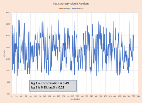
- Random movement around a mean with a strong correlation between successive observations (figure 3)
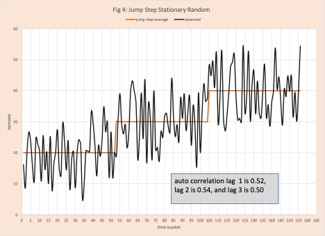
- Random movement around a mean that has a jump step (figure 4)
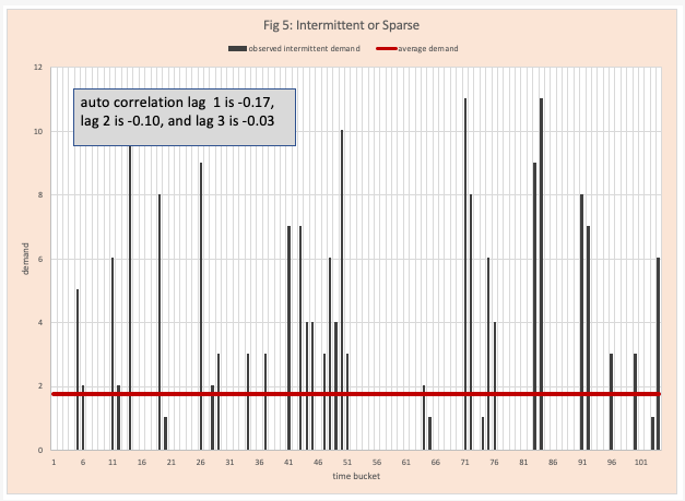
- Intermittent demand (figure 5)
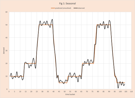
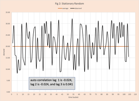
Certainly, any demand planner with experience can look at these visual displays in figures 1 to 5 and classify them; there are too many products for this to be practical. In some cases (for example figures 3 and 4) some interactive help from the local statistician might be needed. Again, not practical. Arkieva’s Swifcast does the heavy lifting. It merges techniques from machine learning and artificial intelligence with an in-depth knowledge of advanced statistics (run tests, error analysis, first-order differencing, lag transformations, autocorrelation, etc.) to quickly make this classification.
An overview of the basic advanced statistical methods is a topic for another time.
Limits of the old classification methods – Machine Learning to the Rescue
In the section “origins of profiling”, we identify that the traditional method involved an old metric called the coefficient of variation (COV). COV = standard deviation / mean. Its original use was in chemistry and engineering. As with many statistical metrics developed for the science side, when applied to the supply chain, its limitations are clear, but its use becomes institutionalized.
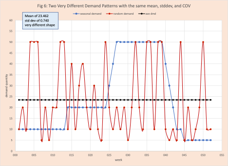
What are its limits? Figure 6 makes this clear. We have two demand patterns with very different shapes. One is clearly seasonal and the second random around a stationary mean. In both cases, the standard deviation and mean (therefore the COV) are the same. As any experienced demand planner will recognize the patterns are very different and this information limitation directly limits the firm’s ability to plan and respond. Clearly, the machine learning-based demand profile will have a positive impact on inventory management.
Conclusion
Machine Learning and automated intelligence combined with deep statistical knowledge imbedded in software with AI methods and the use of advanced optimization can dramatically improve demand forecasting using historical times series data in tactical and operational decision tiers. Most importantly it provides critical insight – this is the best you can do with the data that you have. It can also point the way to additional data needed to improve the forecast, how to assess risk, and how best to monitor and track execution (decision tier relevant time response). One of the critical functions of Swifcast is demand profiling. The new demand profiling function is a substantial improvement over the historic method using coefficient of variation providing critical new insight to support all functions of demand management – this insight is critical to successful supply chain management.
Enjoyed this post? Subscribe or follow Arkieva on Linkedin, Twitter, and Facebook for blog updates.