A view from the trenches – community intelligence
A recent Arkieva Blog, “Effect of Shutdowns (or Other Supply Disruptions) on Demand Variability” does an outstanding job discussing a random effect that can introduce demand variability and computational methods to support planners and managers in handling these such as “metrics of variability”, ignore the zeros, or replace them with the average value across the time bucket neighborhood.
In reading the blog, my immediate thought was “why are shutdown days impacting demand?” Shutdown days are either planned well in advance or inadvertent and unwelcome manufacturing excursion- this is a factory issue, not a demand issue. The answer is simple; in some instances, a firm will use shipments as their demand history. This is simply easier data to collect and store and often a good approximation – especially if your real goal of the demand estimation is to estimate the required output from the factory across products and across time.
Then my attention turned to early lessons in 1978 from Gary Sullivan (IBM) and Gene Woolsey, knowing the details of the application area typically reveal some lessons that make for a better solution. In modern analytics terms this is referred to as the “use of the local domain knowledge” (LDK), Prof. Ed Feigenbaum referred to this as community intelligence.
An example will make this clear. Table 1 is the shipment history, each row is a day of the week, each column is a week, and additionally, we have calculated the total shipments for a week. The organization of the shipment captures the community intelligence whereas the factory has production by week orientation.
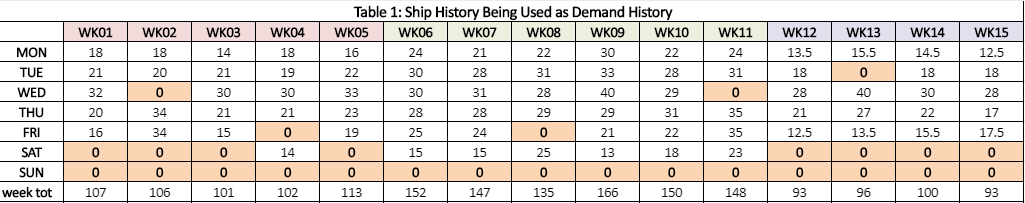
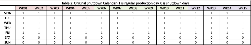
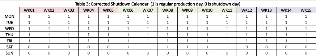
We observe zeros ships for all Sundays, zeros for most Saturdays, and some sporadic zeros across Monday to Friday. We suspect the Saturdays and Sundays are planned shutdown days. We take a trip to see the factory planner and ask for the planned shutdown calendar (Table 2 where 0 is a shutdown day). This shows that every Saturday and Sunday is a shutdown day. When we compare this with the ship data in Table 1, we immediately notice a sequence of “production” Saturdays from WK06 to WK11. We call the factory planner asking about this and she immediately recognizes she has given us the original shutdown calendar (Table 3), not the revised calendar after it was determined production starts would need to increase to meet a surge in demand.
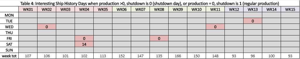
The next step is to identify “shipment values” that are not aligned with the shutdown calendar. These are “interesting days” where the rest are not interesting. A day is interesting if
- There is no shipping (production) (value of 0 in Table 1) on a regular production day (value of 1 in Table 3)
- There is shipping (production) (value > 0 Table 1) on a shutdown day (value of 0 in Table 1)
Table 4 identifies these days of interest where the cell value is not blank. Table 4 also has the total shipments for the week in the last row. Figure 1 has a graph of these values. We have five zero values (which we will assume are sporadic) and one nonzero.
Read more: Lots of Zeroes? Basic Guidelines to Managing Intermittent Demand
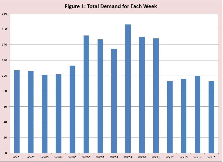
Let’s look at the zero in the cell (WED, WK02). How best to handle this zero? One computational method suggested in the blog on Shutdown Days was to replace the zero with an average value based on the two prior days and two following days. In this situation we would replace the zero with 26.5 = (18 + 20 + 34 + 34)/4. Sounds reasonable! Note this changes the ship sum for WK02 from 106 to 132.5; looking at Figure 1 we see the total weekly ships for WK01 to WK05 is about 105, increasing the weekly total ships (demand) for WK02 well beyond this value. We make a return visit to the factory planner and chat with the factory demand planner (which is a different role than the supply chain demand planner).
After chatting about changes in the cafeteria, she informs us the factory typically gets an estimated demand by week from the business and then allocates it across each of the regular workdays (as defined by the shutdown calendar), where more production is allocated midweek. If the factory is down for the day (the sporadic zero in Table 1), then the factory works to make it up on the following regular days to meet the weekly target. If needed, the factory will work on a weekend day (the regular shutdown days).
After this “community intelligence” lesson, we huddle and conclude
- For now, estimating demand by week is all that is needed as long as the assumption that factory production to meet real exit demand is only needed by the end of the week to use the following week
- It is important to have a central location where the shutdown calendar is stored and available to access.
- It would be helpful to have the allocation percentages the factory uses to assign demand to each day in the week (for example 15%, 20%, 30%, 20%, and 15% for Monday to Friday).
Often a little community intelligence will go a long way in making a computational challenge easier and improving the quality of the solution. Complexity exists whether you ignore it or not, best not to ignore it.