
In this week’s What-if Wednesday post, Arkieva Supply Chain Optimization Consultant – Abhishek Shah – shares the results of a what-if demand forecast simulation using the Winters multiplicative alpha parameter.
The Holt-Winters Multiplicative Method
Until now we had been varying parameters in the Holt-Winters additive method. Starting this week, and in the next few posts, we will run similar simulations using Holt-Winters multiplicative method. Multiplicative is just another variation of the Holt-Winters method where it calculates the seasonal component somewhat differently than the additive method. One would use the multiplicative variant of the Holt-Winters method when the seasonal variations in the data series are proportional to the level of the series. (An Additive method is preferred when the variations are somewhat constant throughout the series.)
Demand Forecasting Method: Holt-Winters Multiplicative Forecast Parameter Simulation – Alpha
The Holt-Winters multiplicative method also has the same three parameters – Alpha, Beta, and Gamma – which determine the relative weighting of recent and more distant history in fitting intercept, trend, and seasonal correction terms. All three parameters range from 0 to 1, with larger values giving more weight to recent history.
- Alpha affects the estimate of the intercept
- Beta affects the trend
- Gamma affects the seasonal correction terms.
We will run simulations by varying the Alpha parameter in this blog post. The charts below show historically observed values from the last three years and forecasts using an Alpha value of 0.05, 0.1, 0.2, 0.4, and 0.8.
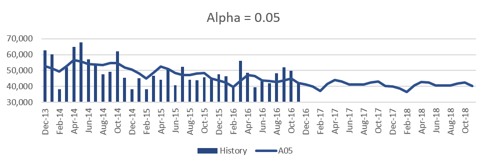
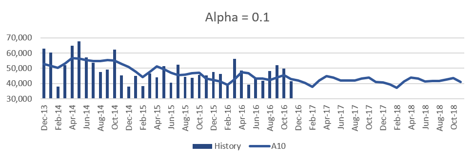
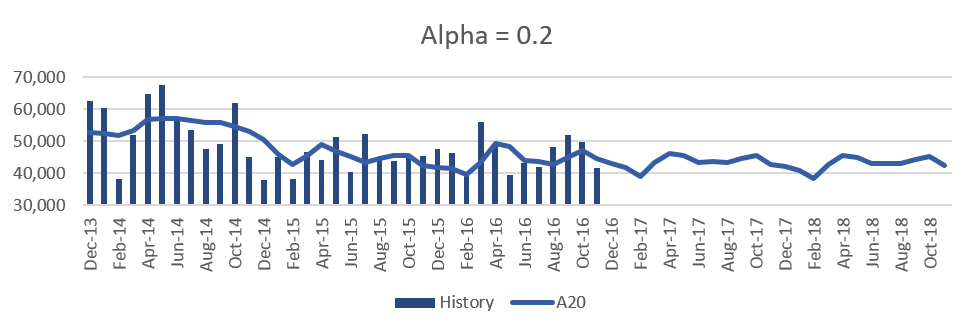
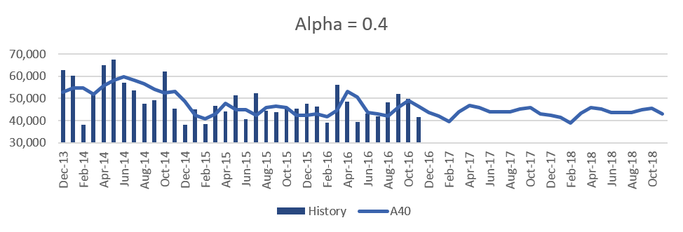
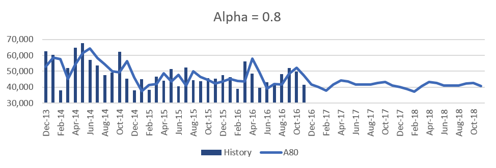
The overall behavior of the forecast with changing alpha is similar to what we saw with the additive method in the previous blog. As we increase the value of Alpha the forecast increases except when the alpha is too high (0.8). One important thing to note with this method: the ups and downs become sharp as we change alpha from 0.05 to 0.8 because the variations are proportional to the level and not constant. You can compare the forecast from the previous method here.
[Related: What-if Wednesday: Forecast Simulation – What Happens if You Change The Alpha Parameter in a Forecasting Method? ]For Feb 2017 as Alpha goes up from 0.05 to 0.4, the forecast increases. This is because the most recent months (Aug-16 – Nov-16) have a relatively higher value than previous months. However, when alpha becomes too high (0.8) we see that the forecast decreases a little bit. This is because almost all (80%) the weightage is on Nov-16 which is lower than the previous months. So too high of an alpha also may not be good in smoothing the forecast unless the business is very sensitive to the most recent history.
Simulation Forecast Numbers

In our next What-if Wednesday post, I will continue this discussion by changing the trend parameter.
In businesses where near term history is significant to the forecast, one can experiment with higher values of alpha. For example, if there has been a significant up (or down) turn in the last 3-5 months and there is the need to influence the forecast heavily towards that turn. Usually, with this method, similar to the additive method, an alpha value between 0.05 and 0.1 is recommended.
Want to join in our What-if-Wednesday posts? Add a comment below or send a tweet to @Arkieva with #WhatifWednesday, or email editor@arkieva.com to suggest a topic, scenario or simulation that you would like us to discuss.
Enjoyed this post? Subscribe or follow Arkieva on Linkedin, Twitter, and Facebook for blog updates.