Summary
In earlier blogs, we covered the importance of profiling the demand history as a critical component of wiser or smarter forecasting to overcome data-driven disasters and pointed to the importance of operations management and community intelligence. There are a number of data analysis “tools of the trade” that have proven effective in exploring data to get it to tell a story. One such method is the first-order difference (FOD). The purpose of this blog is to provide an overview of FOD with respect to profiling demand history.
Introduction
In earlier blogs, we covered the importance of profiling the demand history as a critical component of wiser or smarter forecasting. There are several data analysis “tools of the trade” to explore a data set. Exploratory is a term first coined by John Tukey. One of these is the first-order difference (FOD). The purpose of this blog is to provide an overview of FOD with respect to profiling demand history.
Basics of First Order Difference (FOD)
What is the first-order difference (FOD)? It is the difference between the observation for this time period and the prior time period. Let
- X(t) be the observation for this time period (t)
- X(t-1) be the observation for the prior time period (t-1)
- D(t) be the first order difference between the observation at time i and time (i-1)
D(t)= X(t) – X(t-1)
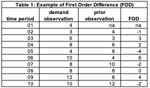
The example in Table 1 will make this clear. We have 10 demand observations (column 2). Column 3 is the demand observation for the prior period. For time period 2, the demand observation is 3 and the demand observation for the prior period (1) is 4. The FOD is 3-4 = -1. Observe there is no FOD for time period 1 since there is no prior time period. For time period 8, the demand observation is 8, and the demand observation for the prior time period (7) is also 8. The FOD is 8-8 = 0.
FOD is an easy calculation in any tool of thought that is orientated toward data analysis. In APL, one of the original programming languages for data analytics, the values would be stored in the vector X and FOD is a direct calculation.
X← 4 3 6 8 4 10 8 8 12 10,
FOD← (-2)-/X.
FOD is -1 3 2 -4 6 -2 0 4 -2
We will explore the power of FOD by examining three common types of series patterns.
Random Variations around a Steady Average Demand
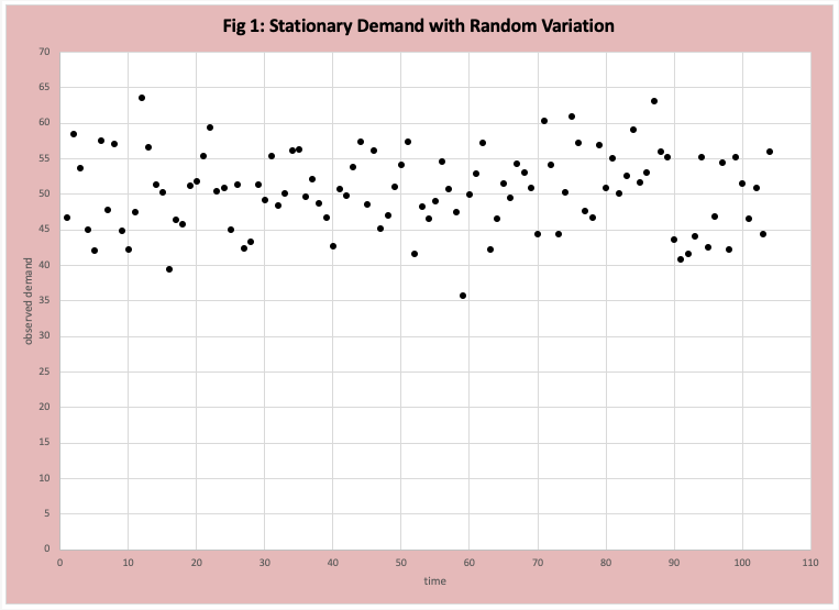
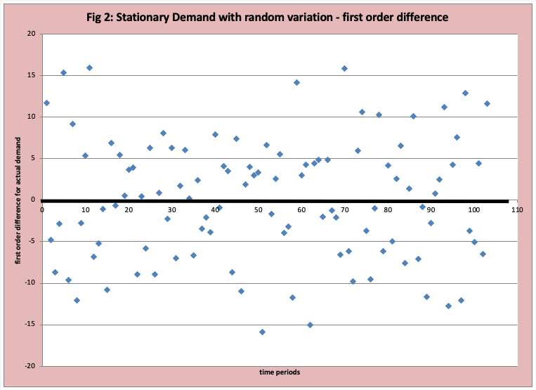
The technical term is a “stationary” time series with random variations. Our example demand data observations for 104 weeks are displayed in Figure 1. At first glance, it is difficult to get a sense of the demand profile. Figure 2 is a graph of the first-order difference (FOD), where a zero line is drawn. If the demand is stationary (no trends, jumps, or seasonal variations), then the pattern should be a random and consistent (stable) distribution of values above and below the ZERO line. At first glance, this is a reasonable assumption. Of course, there are formal data analysis methods to verify if our estimate of “random and consistent” is reasonable. Future blogs will describe these methods (for example the non-parametric run test and autocorrelation). Specific to this data set the mean is 50 and the standard deviation is 6. The errors are normally distributed.
Random Variation around Steady Growth
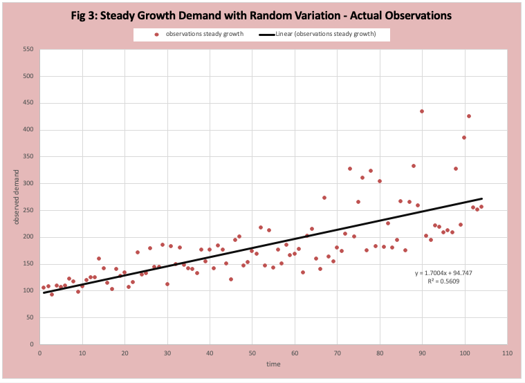
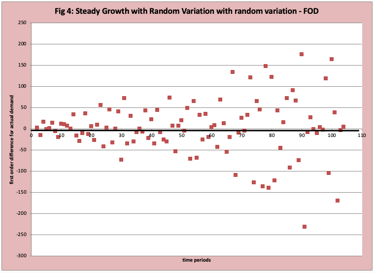
The technical term is stationary growth with random variation. Figure 3 has a scatter plot of the observed data with a “best fit straight line” inserted. It is difficult to interpret Figure 3. Figure 4 has the FOD plot of this data which provides far more insight into the nature of the demand history.
- Early on, the number of observations above and below zero appears to be randomly split with many close to zero.
- Over time the magnitude of the differences is increasing.
- This indicates that there is a reasonably steady growth rate (linear) where the amount of variability increases with time. The “technical statistical term” is the variance (average variation) (it changes over time).
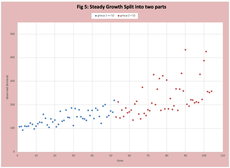
- The variability factor is stronger than the growth rate factor. This can and does hide long-term growth and can drive unnecessary business adjustments, or at minimum the wrong search process. In Figure 5 we adjust the scatter plot in figure 3 to isolate the two years, which makes the increase in variability clearer.
- It also generates the business question that drives this variability.
Seasonal Growth no Growth Random Variation
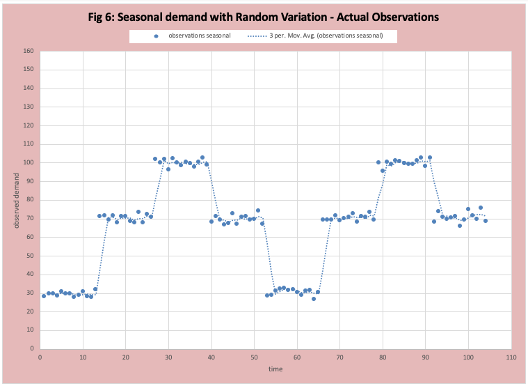
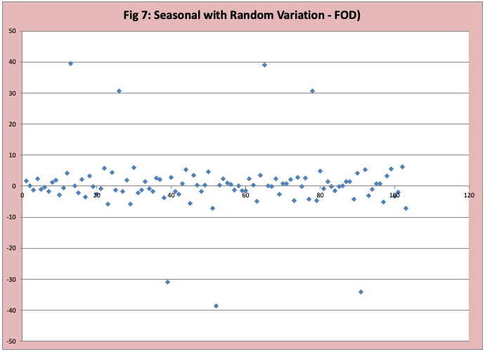
Figure 6 graphs the actual data where there is a seasonal variation that “jumps” and then random variation within the jump. I have also included the 3-period moving average . in this demand pattern where the average demand is different during different groups of weeks. The best known is the Holiday season where demand jumps in November and December and plummets in January and February. In our example we will use ice cream where the average demand for weeks 1 to 13 is 30 (winter), for weeks 14 to 26 is 70, weeks 27 to 39 is 100, and weeks 40 to 52 is 70. There is a random variation around the average. Figure 7 has the FOD graph, we see most data points are scattered around zero, but a few points represent a jump shift up or down in demand.
Conclusion
In previous blogs, we have warned about avoiding data-driven disasters and pointed to the importance of operations management and community intelligence. There are a number of specific methods and methodologies for data analysis developed and applied in earlier times that have proven to be effective in getting the data to tell a story and avoiding disasters. In this blog, we have referred to these as “tools of the trade” of being a successfully applied statistician. In this blog, we have provided some basic information on the simple method known as “first-order difference” (FOD). The first example on stationary times series in figure 1 and 2 make clear the power of this simple method. A later blog will cover the importance of simple, but helpful methods such as the non-parametric run test.
Enjoyed this post? Subscribe or follow Arkieva on Linkedin, Twitter, and Facebook for blog updates.