
Summary
Smart Software’s advanced supply chain analytics exploits multiple advanced methods. Two of the most important are “statistical bootstrapping” and “Monte Carlo simulation”. Since both involve lots of random numbers flying around, folks sometimes get confused about which is which and what they are good for. Hence, this note. Bottom line up front: Statistical bootstrapping generates demand scenarios for forecasting. Monte Carlo simulation uses the scenarios for inventory optimization.
Bootstrapping
Bootstrapping, also called “resampling” is a method of computational statistics that we use to create demand scenarios for forecasting. The essence of the forecasting problem is to expose possible futures that your company might confront so you can work out how to manage business risks. Traditional forecasting methods focus on computing “most likely” futures, but they fall short of presenting the full risk picture. Bootstrapping provides an unlimited number of realistic what-if scenarios.
Bootstrapping does this without making unrealistic assumptions about the demand, i.e., that it is not intermittent, or that it has a bell-shaped distribution of sizes. Those assumptions are crutches to make the math simpler, but the bootstrap is a procedure, not an equation, so it doesn’t need such simplifications.
For the simplest demand type, which is a stable randomness with no seasonality or trend, bootstrapping is dead easy. To get a reasonable idea of what a single future demand value might be, pick one of the historical demands at random. To create a demand scenario, make multiple random selections from the past and string them together. Done. It is possible to add a little more realism by “jittering” the demand values, i.e., adding or subtracting a bit of additional randomness to each one, but even that is simple.
Figure 1 shows a simple bootstrap. The first line is a short sequence of historical demand for an SKU. The following lines show scenarios of future demand created by randomly selecting values from the demand history. For instance, the next three demand might be (0, 14, 6), or (2, 3, 5), etc.
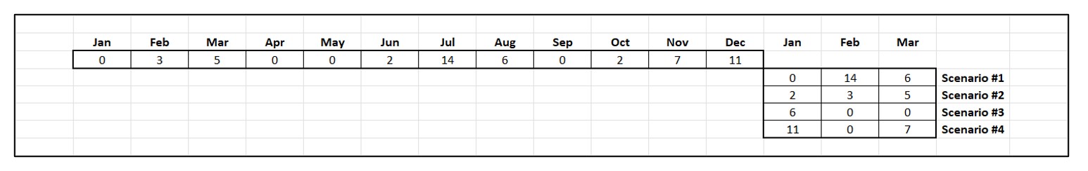
Figure 1: Example of demand scenarios generated by a simple bootstrap
Higher frequency operations such as daily forecasting bring with them more complex demand patterns, such as double seasonality (e.g., day-of-week and month-of-year) and/or trend. This challenged us to invent a new generation of bootstrapping algorithms. We recently won a US Patent for this breakthrough, but the essence is as described above.
Monte Carlo Simulation
Monte Carlo is famous for its casinos, which, like bootstrapping, invoke the idea of randomness. Monte Carlo methods go back a long way, but the modern impetus came with the need to do some hairy calculations about where neutrons would fly when an A-bomb explodes.
The essence of Monte Carlo analysis is this: “Our problem is too complicated to analyze with paper-and-pencil equations. So, let’s write a computer program that codes the individual steps of the process, put in the random elements (e.g., which way a neutron shoots away), wind it up and watch it go. Since there’s a lot of randomness, let’s run the program a zillion times and average the results.”
Applying this approach to inventory management, we have a different set of randomly occurring events: e.g., a demand of a given size arrives on a random day, a replenishment of a given size arrives after a random lead time, we cut a replenishment PO of a given size when stock drops to or below a given reorder point. We code the logic relating these events into a program. We feed it with a random demand sequence (see bootstrapping above), run the program for a while, say one year of daily operations, compute performance metrics like Fill Rate and Average On Hand inventory, and “toss the dice” by re-running the program many times and averaging the results of many simulated years. The result is a good estimate of what happens when we make key management decisions: “If we set the reorder point at 10 units and the order quantity at 15 units, we can expect to get a service level of 89% and an average on hand of 21 units.” What the simulation is doing for us is exposing the consequences of management decisions based on realistic demand scenarios and solid math. The guesswork is gone.
Figure 2 shows some of the inner workings of a Monte Carlo simulation of an inventory system in four panels. The system uses a Min/Max inventory control policy with Min=10 and Max=25. No backorders are allowed: you have the good or you lose the business. Replenishment lead times are usually 7 days but sometimes 14. This simulation ran for one year.
The first panel shows a complex random demand scenario in which there is no demand on weekends, but demand generally increases each day from Monday to Friday. The second panel shows the random number of units on hand, which ebbs and flows with each replenishment cycle. The third panel shows the random sizes and timings of replenishment orders coming in from the supplier. The final panel shows the unsatisfied demand that jeopardizes customer relationships. This kind of detail can be very useful for building insight into the dynamics of an inventory system.
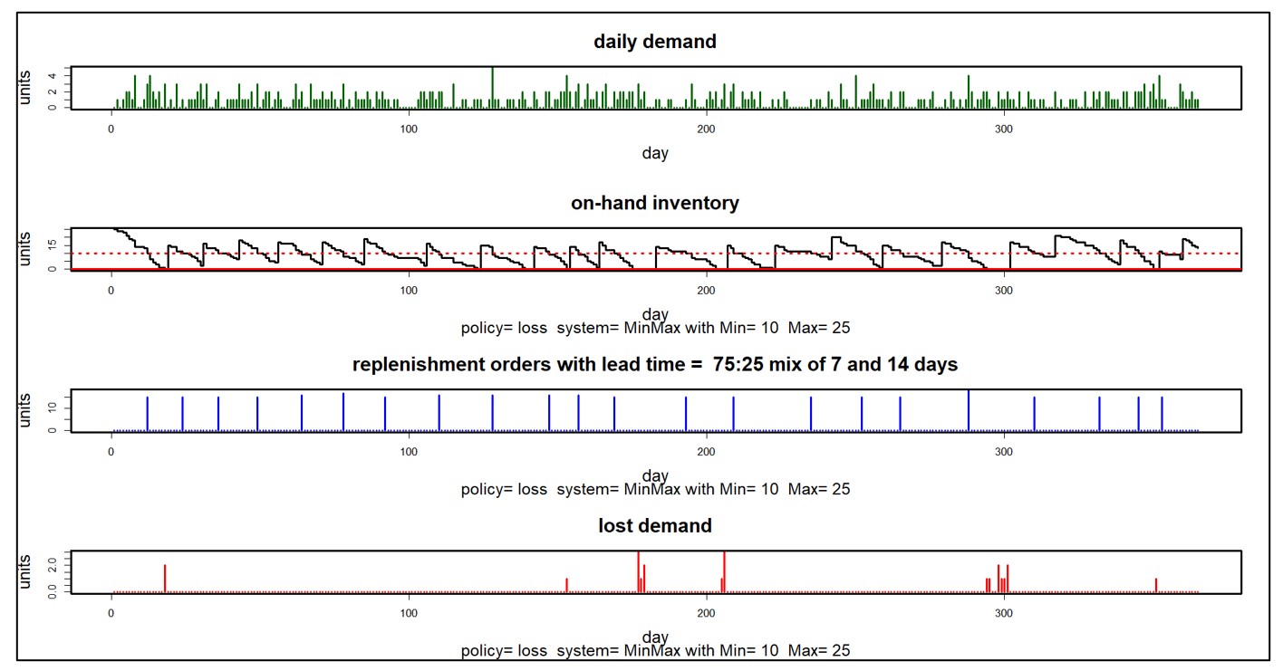
Figure 2: Details of a Monte Carlo simulation
Figure 2 shows only one of the countless ways that the year could play out. Generally, we want to average the results of many simulated years. After all, nobody would flip a coin once to decide if it were a fair coin. Figure 3 shows how four key performance metrics (KPI’s) vary from year to year for this system. Some metrics are relatively stable across simulations (Fill Rate), but others show more relative variability (Operating Cost= Holding Cost + Ordering Cost + Shortage Cost). Eyeballing the plots, we can estimate that the choices of Min=10, Max=25 leads to an average Operating cost of around $3,000 per year, a Fill Rate of around 90%, a Service Level of around 75%, and an Average On Hand of about 10
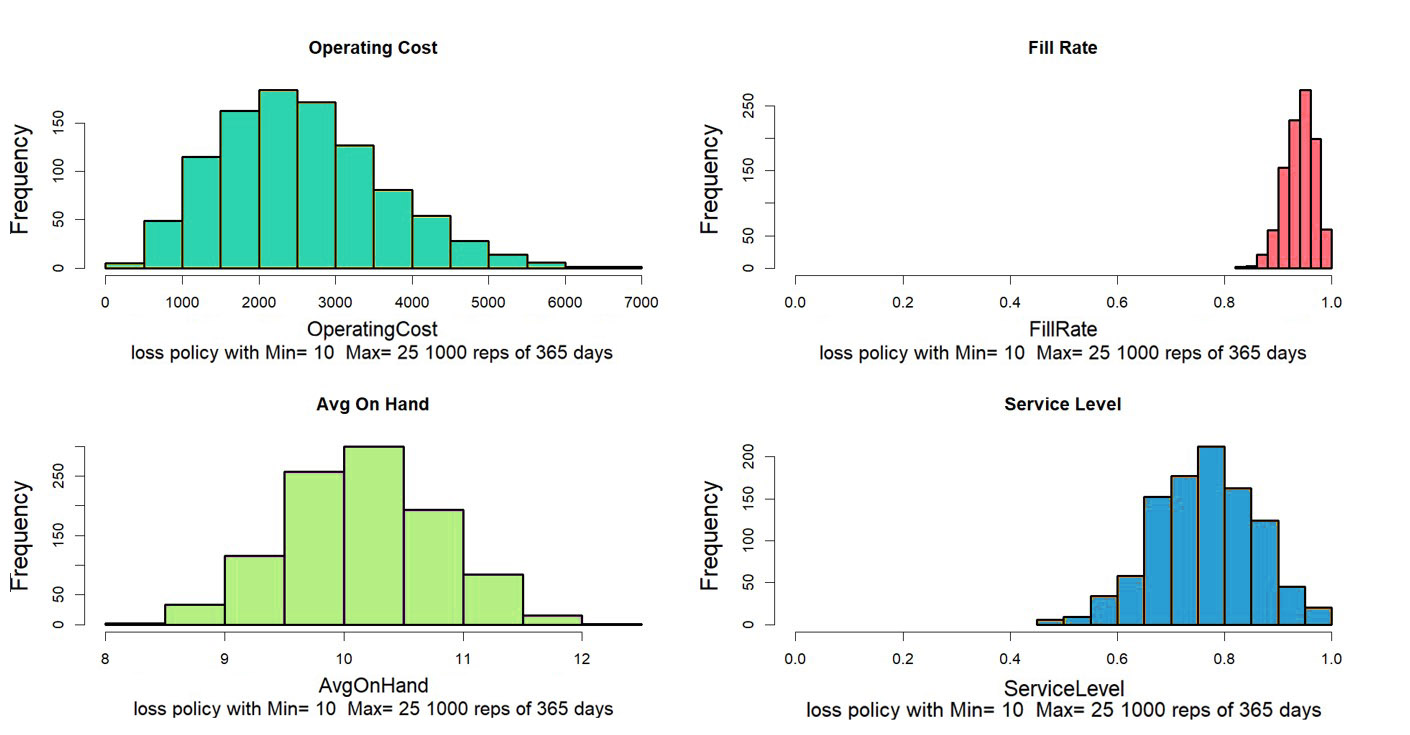
Figure 3: Variation in KPI’s computed over 1,000 simulated years
In fact, it is now possible to answer a higher level of management question. We can go beyond “What will happen if I do such-and-such?” to “What is the best thing I can do to achieve a fill rate of at least 90% for this item at the lowest possible cost?” The mathemagic behind this leap is yet another key technology called “stochastic optimization”, but we’ll stop here for now. Suffice it to say that Smart’s SIO&P software can search the “design space” of Min and Max values to automatically find the best choice.