
The bullwhip effect is one of the common problems of supply chains, affecting manufacturers, distributors, and retailers alike.
The cause of the bullwhip effect is difficult to recognize in a large, rapidly growing company. Pay attention to the symptoms. Some of the most common are raw materials, finished products, stock outs, and over stocks.
Such an ambivalent state of stocks does not allow the company to use its resources in full. The idea of balancing the system in the current conditions seems difficult to achieve.
Let’s start the problem analysis with retail. Generally, when forecasting sales for the period between deliveries and analyzing the accuracy of previous demand, a safety stock is calculated, which is a percentage of sales for the forecast period. In other words, the bigger forecasted sales are, the more mistakes they contain, and the bigger safety stock should be.
Unpacking Bullwhip Effect Examples
Sales forecast for the period = 1 pallet. Safety stock = 50% of demand forecast for the period. Balance at the beginning = 0 pallets. Order = sales forecast + safety stock – current stock. The order is rounded to pallets.
In the first week, we order 1+(0.5*1) – 0 (balance) = 1.5 pallets. But since it is necessary to place an order in multiples of a pallet, it is equal to 2 pallets. Actual sales turned out to be lower than forecasted by 20% or 0.8 pallets. Balance at the end of the period: 2- 0.8 = 1.2 pallets.
In the second week, we recalculated the sales forecast. Now it is 0.8 pallets. We calculate the order again: 0.8 + (0.5 * 0.8) – 1.2 (balance) = 0. We do not place an order. The current stocks will cover the projected sales and forecast error. But actual sales appeared higher than forecasted, and we sold 1.2 pallets.
In the third week we’ll order 2 pallets again.
How accurate are your forecasts? Obviously, the scale of the problem is far beyond the issue with the forecast.
If the company is just starting to work on the forecast, then by improving the accuracy of the forecast, it’s possible to slightly reduce the level of safety stocks. The management then sets the goal to improve the forecast constantly. But the fact is that improvement has its own limits and feasibility. If the cost of calculating the forecast exceeds the profit, then it becomes useless.
But, even if the goal is achieved, after increasing the accuracy of the forecast, there remains a “system error” of multiplying sales fluctuations further down the supply chain. This approach may show improvement but does not solve the original problem.
Let’s consider how this affects the distributor who receives our orders (2.0 and then 2 pallets). Naturally, the distributor has many retailers. The order logic remains the same for everyone. A company must keep much more stock as fluctuation amplitude is bigger (e.g. from 0 to 30 pallets).
As it’s known from the previous example, a retailer order from a distributor is not exactly a demand. Rather, it is a rough estimate of future sales, distorted by the conditions of purchase and incorrect purchases in the past.
In order to cover such fluctuations in demand, the manufacturer needs to constantly store at least 30 pallets of goods, since it is not known when and what amount is going to be an order from the distributor. It must be considered that manufacturers have dozens, or even hundreds of such customers.
In addition, it is impossible to produce 30 pallets at any time, since the manufacturer has its own limitations that cannot be ignored. For example, equipment capacity, scheduling intervals, optimal order quantity, long lead times, sequencing constraints, etc.
If the optimal or economic order quantity makes up 100 pallets, then the manufacturer will keep a stock from 0 to 100 pallets.
After the production of the optimal batch size, the stock of products becomes more than needed. In this case, within a few weeks of the planning horizon, as a rule, something will not go according to plan. An urgent order will appear from the sales department, equipment will break down, there will be an unexpected peak in demand for one of the manufactured products, etc. Any event that will shift the production schedule. There is a high probability that when the manufacturer receives an order from distributors, the products will not be produced in time. Therefore, the manufacturer, as well as the retailer, will increase its safety stocks, which will lead to an additional increase in orders and lengthening the periods of no orders, which means that information about real demand will be distorted even more.
As a result, a “bullwhip effect” will appear in the supply chain. This is a situation when even the smallest deviations and fluctuations in the supply chain lead to uncontrolled significant changes on its other end.
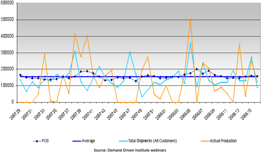
Perhaps the example of stock fluctuations in the retailer-distributor-manufacturer supply chain seems overly simplified. Below is a graph of a stable selling product from the FMCG market.
A high level of inventory is needed to smooth out acute problems and create reliability illusion. But it does not solve the problem of stock fluctuations from artificially high levels to shortages since this is a natural consequence of planning on distorted information.
The bullwhip effect is an old phenomenon. Earlier it was believed that the problem would be solved with powerful computing technology, which would allow storing and processing large amounts of data. Despite the fact that today we have many tools for processing and storing data, the problem has not gone away, but, on the contrary, has even worsened. The product range is growing, the life cycle is decreasing, the variability of demand is less and less predictable. It becomes obvious that we need to radically revise the approach to supply chain management. This is the task that the DDMRP methodology covers.
Eliminate the Bullwhip Effect with DDMRP
The key inventory management tool in DDMRP is the buffer. The buffer consists of 3 zones: red, yellow and green. Each zone has its own purpose and calculation logic.
The red zone is a flow safety and is designed to protect against variability.
The yellow zone is a “cycle stock” that provides consumption for the replenishment time.
The green zone is a flow controller. It includes all sorts of logistical restrictions and determines the average order and how often it will be generated. And all together they make up a buffer.
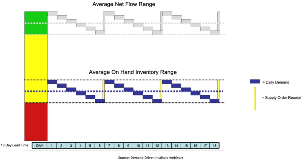
The graph shows the fluctuation of the information flow (Average Net Flow Range), which is responsible for the information transfer further along the supply chain without distortion.
At the bottom of the yellow zone, the physical flow will fluctuate by the size of the green zone (Average on Hand Inventory Range). Thus, the system is initially set up to allow neither out of stocks nor over stocks. Using a buffer according to this methodology helps all links of the supply chain to cover problems with boost in sales and respond in time to drops in demand. It also provides an opportunity to balance orders and make them regular.
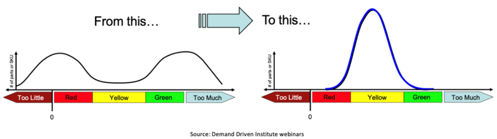
The graph shows how the nomenclature distribution looks before and after the use of the methodology. On its left side we see a bimodal distribution of stocks, this example is described at the beginning of the article. There are lots of stocks, sometimes none at all. The optimal state of stocks in such management is an exception to the rule. The right side of the graph shows that there can be stock outs and over stocks, but most of the stocks are kept in the optimal range.
In summary, no matter where your company is in the supply chain, the “whip effect” affects everyone. The supply chain needs to be balanced. The DDMRP methodology will help to cope with this problem.