Historically, most of the key planning and computational activities (models, time series, machine learning, and other analytics) that support extended supply chain management (SCM) are “deterministic models”. That is, they use a single estimated value for key information (examples: demand for a product in a period, capacity available for a resource, production output for a period, lead or cycle time for a production or shipment action, yield, etc.) in the computational and planning activities. Certainly, executives, planners, and analytics professionals are aware that the events are not deterministic but stochastic (uncertainty or variability – managing risk). There is a growing effort to handle this variability in planning modules. Two terms that are often heard in demand management are probabilistic forecasting and confidence intervals. The purpose of this blog is to shed some light on these concepts.
- A probabilistic forecast involves the identification of a set of possible values and their probability of occurrence for the actual demand for a product (or groups of products) in a specific time period. It is focused on the specific event. In statistics, this is a probability distribution (density) function – a PDF.
- A confidence interval (in the traditional sense) involves identification of a set of possible values their probability of occurrence for the average demand for a product in a specific time period. It is focused on the average or expected value if the “arrival of demand” was repeated many times. If certain conditions are met in the data and demand structures, then the normal distribution (a bell-shaped curve) can be used to calculate this interval.
Read More: What’s the Core purpose of Supply Chain Management?
As always in statistics, an example will make this much easier to understand. Let’s assume we run a local ice cream production facility (my first demand planning job in 1972) that only operates during the summer (20 weeks) and a critical component of managing our business is generating an estimating demand by a week in March. For simplicity we will assume there are no seasonal factors during the summer (more demand in July than in June for example), no special events (for example a two for one special on July 4th), no need or value in using a long term weather forecast, and no trends. There is variability in weekly demand that does not appear to be predictable. Since the Great Pumpkin is a close friend, it has given us the probability of demand each week in Table 1 and Figure 1.

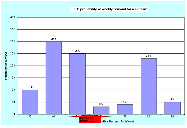
In statistics terms Table 1 is the probability distribution (density) function (PDF), it simply tells us the possible values for demand and the probability of each possible demand. The sum of the probabilities must be 100%. The average or expected demand is 55. This is the sum of each demand times its probability. 55 = (30 x .1 + … +90 x .05). This formula is from basic probability. The standard deviation (STDDEV) is 18.7; this is a measure of the average variation in demands. Figure 1 illustrates the most likely demand are 40, 50 and 80 – called bimodal. Hardly bell or normal shaped. The PDF is the probabilistic forecast for weekly demand for ice cream. We see probabilistic forecasting is a basic concept from probability – conceptually no different than estimating the probability of rolling a seven when throwing two dice or the probability of getting an ace when drawing a card from a deck. The real challenge is creating a great pumpkin to figure out the PDF and then how to use this information.
Before going to the confidence interval example, we need to look at a few important statistics “details”. A standard assumption in statistics and probabilistic forecasting is independent and identically distributed (IID). Simply that the demand this week is independent of the demand last week and the probability (PDF) of demand is the same from week to week (stationary). IID makes the computation easier and at times is a reasonable assumption. Sometimes it is a terrible assumption, but that is a different blog. If we assume IID, this empowers the central limit theorem and enables us to the traditional method to estimate a confidence interval. Just tuck this away as “need to be careful”.
A confidence interval uses sample information to calculate a range of values where population average is likely to occur. In demand planning a sample would be historical data. Assume the data available to me in 1973 was five years of history (Table 2). I generated this using the Monte Carlo process applied to the real probabilistic forecast.
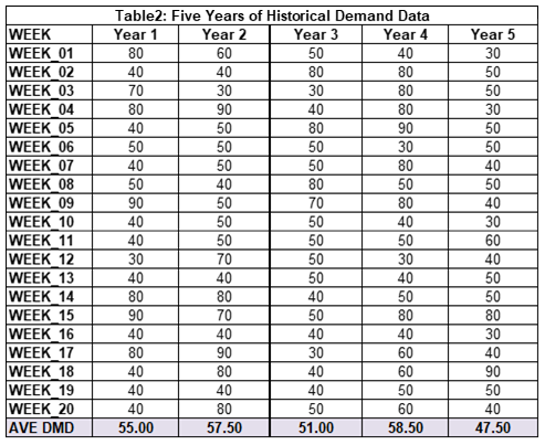
Having just completed my first class in probability and statistics at St. Thomas Aquinas College, I immediately calculated the summary statistics sample average and standard deviation (Table 2).
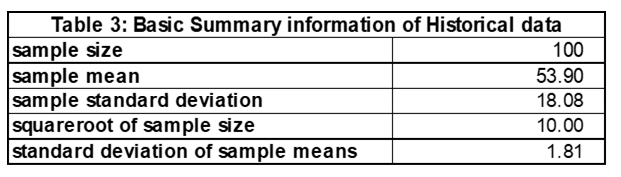
We see the average weekly demand from this sample of size 100 is 53.90 with a standard deviation of 18.08. Having just studied confidence intervals (CI), I calculated some using the formula n.
- (x bar) is the sample average = 53.9
- s is the sample standard deviation = 18.08
- n is the same size = 100
- is the sample mean standard deviation = 1.81
- α is the risk that the actual population mean is not in the confidence interval, (1-α) is the confidence that the actual population mean is in the interval. Typical confidence values are 90% and 95%, where the corresponding alpha are 10% and 5%
- Z is the standard normal distribution (bell shaped curve), it converts the risk (α) into value that makes the interval longer for less risk and shorter for more risk. The most famous value is 1.96 for a 95% confidence interval. In Excel use the NORMSINV build in function.
Some specific examples (Table 4) will make this much easier to follow.
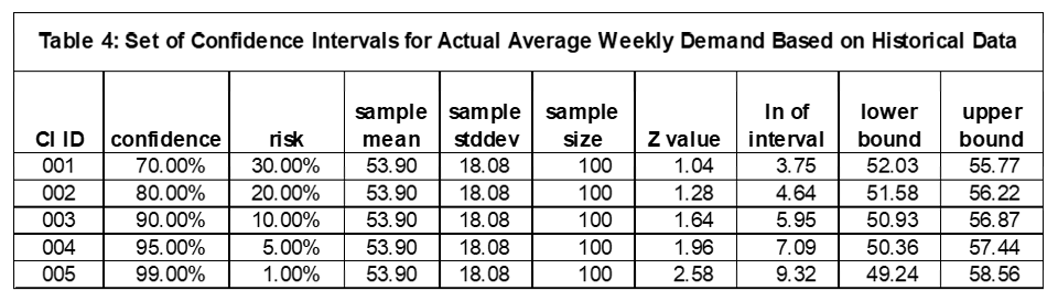
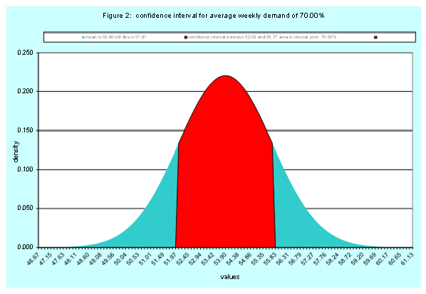
The first confidence interval is (CI ID = 1) is a 70% confidence interval with the lower bound of 52.03 and upper bound of 55.77. In layman terms there is a 70% chance the actual average demand per week is between 52.03 and 55.77. There is a 15% chance the actual average weekly demand is less than 52.03 and greater than 55.77. Figure 2 has a graph of this confidence interval.
Read More: Demand Forecasting Analytical Methods
The fourth confidence interval (figure 3) is the famous 95%. For this data set we are 95% certain the actual weekly average demand falls between 50.36 and 57.44. There is a 2.5% chance the actual average is below 50.36 and a 2.5% chance it is above 57.44. Observe as my confidence increases, the length of the interval increases. There are no free rides.

How does this information help us? If the primary purpose of our demand forecast is to get a quality estimate of the average demand per week, then the 95% interval of [50.36 and 57.44] is very helpful. If we have enough production to produce 60 units per week, then we can be confident on average we can meet demand. If our production capability is only 56 units, then we make an initial estimate of the risk of not having enough production capacity as 15%.
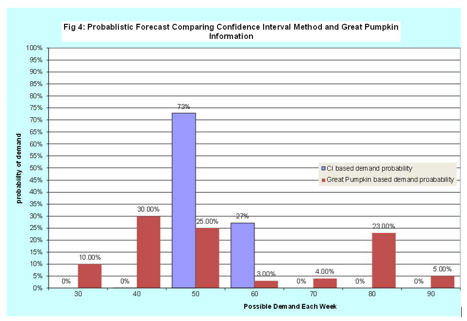
However, the confidence interval is not a probabilistic forecast of actual weekly demand, even though it contains some probability. We can, with a bit of programming and an understanding of the normal distribution, create a PDF based on the confidence interval formula in the format matching the probabilistic forecast provided by the Great Pumpkin. Table 5 and Figure 4 have the probabilistic forecast generated from confidence intervals (CI) compared to the Great Pumpkin (GP) probabilistic forecast.
With a brief glance, we see the average values are close, but the shapes are different. The CI method is much narrower than the GP – essentially missing the weeks with demands of 80. Which is correct? In our case we know the GP is correct, since this was the assumption we made, we generated historical data from this PDF, and then applied the basic concepts of confidence intervals from any introductory statistics class (in my case in 1973, I then went on and took 12 more as well as doing applied work in this area – hardly making for great conversation at social gatherings).
Why the difference? This will be covered in upcoming blogs. Two primary reasons are
- Confidence intervals are focused on the average weekly demand. The probabilistic forecast from GP is focused on individual weekly demands. Here a concept of a prediction interval is needed.
- Confidence intervals use a normal distribution based on the central limit theorem (the 8th wonder of the world.
These both sound subtle or theoretical, but both are critical. As always, the right answer is based on the business need – understanding average (total) demand or the actual variation in demand.
Hopefully this material provides a bit of insight into a reasonably complicated area. A closing thought from Peter Lyon (IBM retired) who was the director of Strategic Systems and led the complete transformation of IBM’s supply chain management process a while back which Arkieva was heavily involved in.
“Complexity exists, whether you ignore it or not – best not to ignore it” – Peter Lyon.