Summary
One of the two fundamental activities in supply chain management is Demand Management (DM). A critical component of DM is estimating future demand. Typically, the only helpful data is demand history (often ship history). This data set is referred to as time series. Quality time series forecasting is a critical component of any successful DM. In this blog we will briefly cover some key insights for successful time series forecasting:
- Profiling the Shape of the Curve is the first stage, and the first step is assessing if the time series is stationary.
- The forecast method identified must capture the shape and be able to project the shape across time.
- There are limits in historical and no amount of “fancy math” can overcome them.
Additionally, we identify some rules of thumb that are often cited and embarrassingly wrong.
Introduction
One of the two fundamental activities in supply chain management is Demand Management (DM), the other is Central Planning. A critical component of DM is estimating future demand. Typically, the only helpful data is demand history (often ship history). This data set is referred to as time series. Figure 1 has a time series of 3 years of umbrella sales in monthly buckets for marketing region 1 (MR1). The goal of the demand planner, in this case, is to estimate umbrella demand in year 4 for MR1. In this blog, we will not address the critical question of what level to forecast or how to combine levels in a pyramid (product/region into product). The initial estimate displayed is the average monthly sales across the three years of history.
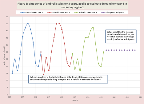
The purpose of time series forecasting methods is to identify patterns (trend up or down, seasonal (cyclical), jumps, autocorrelations (yesterday has a strong influence on today), etc.) in the historical data that is helpful to understand the demand and use these to estimate future demand under the assumption that past applies to the future. No matter how sophisticated your methods, this is all you can mine from time-series data.
In this blog, we will provide a quick overview of time series forecasting, offer some rules of thumb, and identify some rules of thumb that are embarrassingly wrong.
Characterizing the shape is the starting point.
This is step 1 and the first shape is called “boring” or stationary. The demand per time bucket varies randomly around a mean (Figure 2). It is critical to use some advanced methods (such as run test or binomial) to ensure the variation is random. Figure 3 is an example of a stationary time series with too much variation to be random.
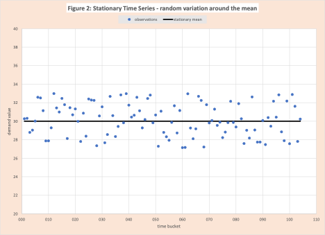
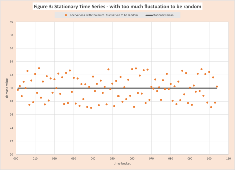
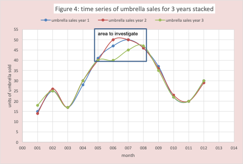
Figure 4 stacks the historical data for umbrella sales to make clear the repeatable pattern across time. Computationally we would use autocorrelation to find this. For this data set, the autocorrelation for lag 12 is 97%. Lag 1 is 66%.
Identifying a forecasting method
In step 2 we search for a curve that captures the shape of the historical data and can be used to estimate the future. Find the curve includes which curve structure and the parameter that gives the best fit possible for the selected curve. Figure 5 displays the result of fitting a two-period moving average to the original data, that fit is a decent fit – not surprising since the lag 1 autocorrelation is 66%. However, it does not contain any information to estimate out in time except repeating the last value.
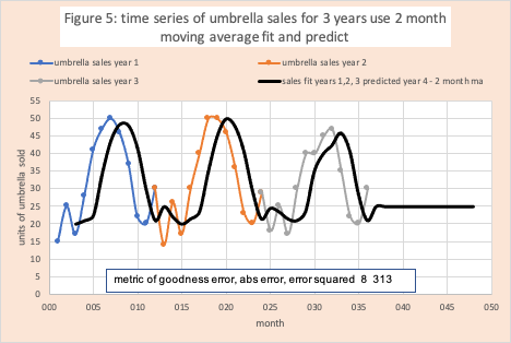
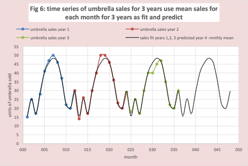
Figure 6 displays the result of fitting a simple cyclical curve where the fit value is the monthly average across the three years (estimate for January is average of Jan01, Jan02, and Jan03). The estimate for each month in year 4 is this monthly average. Observe this as a very good fit – not surprising since the lag 12 autocorrelation is 97%.
Understanding the limits of the historical data you have.
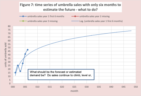
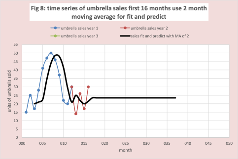
There is an old saying you cannot squeeze water out of rock. No matter how sophisticated your methods, a lack of data limits the insight possible. Using the umbrella data, if we only had 6 months of data (Figure 7), it would be impossible to determine the pattern obvious when we have 3 years of data. Figure 8 has a graph with only 16 data points. If used the first 12 to fit a curve and the last 4 to predict (verify), we could easily conclude moving average was the best fit and miss the entire cyclical pattern.
Using your insight about shape to ask important questions.
In figure 4 the sales pattern has stable repeatability. However, it is clear there is a good amount of difference between the three years in months 6 and 7. Especially for the most recent year (year 3). It is worth asking why and perhaps looking at supporting data: the amount of rain, change in advertising, more competition. There are no magic bullets to extract any additional insight from the historical data for this question. This is the best you can do. At this point, one needs to rely on community intelligence.
Simple Methods are not forecasting methods
Methods such as moving average (MA) and exponential smoothing were not initially created to estimate the future but were for smoothing the bumps in existing data. Business folks, ever on the lookout to simplify a situation to match their computational skills made these forecasting methods. Every business analytics course has a chapter on forecasting that covers MA, exponential smoothing, simple linear regression, and perhaps another method. In time series forecasting classes taken by statisticians, these methods are covered in the first few pages of the book with respect to basic data analysis. As noted earlier the appropriate method is to assess if the time series is stationary – never mentioned in business statistics.
Rules of Thumb that are embarrassingly wrong
- The coefficient of variation (COV) is a metric that will tell you a historical data set is forecastable or not. The COV for the very predictable umbrella sales is 37%. In fact, COV was originally developed for chemistry. The business statistics folks grabbed and ran with it without thought.
- If your only purpose is “fit” historical data, then just use the existing history as is – missing entirely the importance of shape.
- Use simple methods whenever you can – without mentioning stationarity.
- For truly intermittent data, using traditional point forecasting approaches is a fool’s errand.
Conclusion
Quality time series forecasting is a critical component of any successful DM. In this blog we briefly cover some key insights for successful time series forecasting: (a) Profiling the Shape of the Curve is the first stage, and the first step is assessing if the time series is stationary. (b) The forecast method identified must capture the shape and be able to project the shape across time. (c) There are limits in historical and no amount of “fancy math” can overcome them.