
Our customers have usually settled into one way to manage their service parts inventory. The professor in me would like to think that the chosen inventory policy was a reasoned choice among considered alternatives, but more likely it just sort of happened. Maybe the inventory honcho from long ago had a favorite and that choice stuck. Maybe somebody used an EAM or ERP system that offered only one choice. Perhaps there were some guesses made, based on the conditions at the time.
The Competitors
Too seldom, businesses make these choices in haphazard ways. But modern service parts planning software lets you be more systematic about your choices. This post demonstrates that proposition by making objective comparisons among three popular inventory policies: Order Up To, Reorder Point/Order Quantity, and Min/Max. I discussed each of these policies in this video blog.
- Order Up To. This is a periodic review policy where every T days, on-hand inventory is tallied and an order of random size is placed to bring the stock level back up to S units.
- Q, R or Reorder Point/Order Quantity. Q, R is a continuous review policy where every day, inventory is tallied. If there are Q or fewer units on hand, an order of fixed size is placed for R more units.
- Min, Max is another continuous review policy where every day, inventory is tallied. If there are Min or fewer units on hand, an order is placed to bring the stock level back up to Max units.
Inventory theory says these choices are listed in increasing order of effectiveness. The first option, Order Up To, is clearly the simplest and cheapest to implement, but it closes its eyes to what’s going on for long periods of time. Imposing a specified passage of time in between orders makes it, in theory, less flexible. In contrast, the two continuous review options keep an eye on what’s happening all the time, so they can react to potential stockouts quicker. The Min/Max option is, in theory, more flexible than the option that uses a fixed reorder quantity because the size of the order dynamically changes to accommodate the demand.
That’s the theory. This post examines evidence from head-to-head comparisons to check the theory and put concrete numbers on the relative performance of the three policies.
The Meaning of “Best”
How should we keep score in this tournament? If you are a regular reader of this Smart Forecaster blog, you know that the core of inventory planning is a tug-of-war between two opposing objectives: keeping inventory lean vs keeping item availability metrics such as service level high.
To simplify things, we will compute “one number to rule them all”: the average operating cost. The winning policy will be the one with the lowest average.
This average is the sum of three components: the cost of holding inventory (“holding cost”), the cost of ordering replenishment units (“ordering cost”) and the cost of losing a sale (“shortage cost”). To make things concrete, we used the following assumptions:
- Each service part is valued at $1,000.
- Annual holding cost is 10% of item value, or $100 per year per unit.
- Processing each replenishment order costs $20 per order.
- Each unit demanded but not provided costs the value of the part, $1,000.
For simplicity, we will refer to the average operating cost as simply “the cost”.
Of course, the lowest average cost can be achieved by getting out of the business. So the competition required a performance constraint on item availability: Each option had to achieve a fill rate of at least 99%.
The Alternatives Duke it Out
A key element of context is whether stockouts result in losses or backorders. Assuming that the service part in question is critical, we assumed that unfilled orders are lost, which means that a competitor fills the order. In an MRO environment, this will mean additional downtime due to stockout.
To compare the alternatives, we used our predictive modeling engine to run a large number of Monte Carlo simulations. Each simulation involved specifying the parameter values of each policy (e.g., Min and Max values), generating a demand scenario, feeding that into the logic of the policy, and measuring the resulting cost averaged over 365 days of operation. Repeating this process 1,000 times and averaging the 1,000 resulting costs gave the final result for each policy.
To make the comparison fair, each alternative had to be designed for its best performance. So we searched the “design space” of each policy to find the design with the lowest cost. This required repeating the process described in the previous paragraph for many pairs of parameter values and identifying the pair yielding the lost average annual operating cost.
Using the algorithms in Smart Inventory Optimization (SIOTM) we made head-to-head-to-head comparisons under the following assumptions about demand and supply:
- Item demand was assumed to be intermittent and highly variable but relatively simple in that there was neither trend nor seasonality, as is often true for service parts. Daily mean demand was 5 units with a large standard deviation of 13 units. Figure 1 shows a sample of one year’s demand. We have chosen a very challenging demand pattern, in which some days have 10 to even 20 times the average demand.
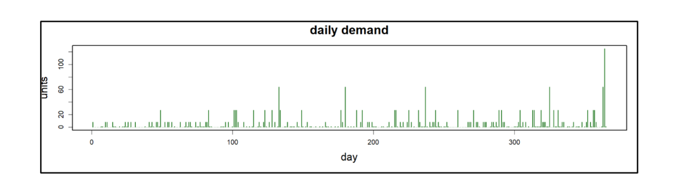
Figure 1: Daily part demand was assumed to be intermittent and very spikey.
- Suppliers’ replenishment lead times were 14 days 75% of the time and 21 days otherwise. This reflects the fact that there is always uncertainty in the supply chain.
And the Winner Is…
Was the theory right? Kinda’ sorta’.
Table 1 shows the results of the simulation experiments. For each of the three competing policies, it shows the average annual operating cost, the margin of error (technically, an approximate 95% confidence interval for the mean cost), and the apparent best choices for parameter values.
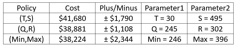
Table 1: Results of the simulated comparisons
For example, the average cost for the (T,S) policy when T is fixed at 30 days was $41,680. But the Plus/Minus implies that the results are compatible with a “true” cost (i.e., the estimate from an infinite number of simulations) of anywhere between $39,890 and $43,650. The reason there is so much statistical uncertainty is the extremely spikey nature of demand in this example.
Table 1 says that, in this example, the three policies fall in line with expectations. However, more useful conclusions would be:
- The three policies are remarkably similar in average cost. By clever choice of parameter values, one can get good results out of any of the three policies.
- Not shown in Table 1, but clear from the detailed simulation results, is that poor choices for parameter values can be disastrous for any policy.
- It is worth noting that the periodic review (T,S) policy was not allowed to optimize over possible values of T. We fixed T at 30 to mimic what is common in practice, but those who use the periodic review policy should consider other review periods. An additional experiment fixed the review period at T = 7 days. The average cost in this scenario was minimized at $36,551 ± $1,668 with S = 343. This result is better than that using T = 30 days.
- We should be careful about over-generalizing these results. They depend on the assumed values of the three cost parameters (holding, ordering and shortage) and the character of the demand process.
- It is possible to run experiments like those shown here automatically in Smart Inventory Optimization. This means that you too would be able to explore design choices in a rigorous way.